This is an updated version of an article originally published in 2015. I only remembered it today, which is useful I hope, given that teachers now have to determine exam grades.

Help is at hand...
Imagine this. You have to mark and assign grades to the two classes of students you teach. That's 60 students. Your colleagues each have to do the same. You, as the head honcho, are responsible for the whole shebang: making sure the marks are in, grades awarded, and reports to parents out. All in the next week or two.
And, you do get time off timetable to do it all, right?
Yes, that’s what I thought….
A few years ago, finding myself in exactly this position, I devised a simple but effective grade predictor in Excel (although you could use any spreadsheet that has a lookup function), for use with mock exams.
What the grade predictor is not
But before I explain how it works, let me state what it is not meant to be. I never intended the system to be a substitute for the teacher's skill of interpretation. However, there is one fact and one assumption I brought to bear on the situation.
The fact was that we knew what the approximate grade boundaries were, as laid down by the examination board. For example, a mark of 70% or above would most likely result in a grade 9, whereas a mark of around 55 would probably deliver a grade 4.
I realise that this is not always the case now, but it was then. If the exams you're entering your students for have grade boundaries that you know in advance, the spreadsheet should be useful. Information about the grade boundaries appears to differ depending on which exam board (awarding body) you use. At least one is going to announce the boundaries on results day! There is some information from the DfE about this. However, you may have to make an educated guess. Bear in mind that the grade predictor I created is really designed to highlight completely unexpected results. For example, if you think a student is grade 8 material, but according to their mock exam results or coursework marks they are predicted to attain a grade 3 — or vice-versa — then that needs investigating. Either your evaluations are wildly optimistic/pessimistic, or they have had some terrible issues in their private life (or cheated). These points are covered below as well, but I just wanted to highlight them up front.
The assumption was that if you were to draw up a grid or table depicting these relationships between marks and grades, so that you could look up a student's mark and then derive their grade by reading across to the next column, in most cases this mechanical approach would be accurate (insofar as this sort of thing can be "accurate", of course).
However, in my experience there are always a couple of what I call "rogue results", or what some people call "outliers" : unexpected results which merit further investigation. For example, Mary has been doing well in all her assignments for the whole year, and contributes productively to class discussions. Then in the trial or mock examination she totally flunks it, obtaining a mark of 12, and even that was partly for spelling her name right. Does that mean your judgement was completely out all this time? A far more reasonable explanation is that something happened to cause this aberration.
So you talk to Mary and discover that the night before she watched a TV program that prevented her sleeping, or that she had a particularly bad attack of exam nerves. In that case, a much fairer approach would be for you to record her grade as predicted by the grid, but then override that, in effect, with a higher grade, making sure to include an explanation as to why you've taken that action.
You cannot just leave the matter there, of course. You and Mary, with the co-operation of her family, have to try and make sure there's not a recurrence in the real exam, when she will not, of course, be given the benefit of the doubt. But it's a good compromise for now because it is being honest in saying what could happen, but establishing the foundation for a report based on what should have happened.
Conversely, Johnny has never shown the slightest interest in the subject, has never scored more than 5% on any assignment -- at least, those few he has actually handed in -- and yet he gains a mark of 98%. I think you will agree that something is amiss. Either he was incredibly lucky in terms of the questions that came up on the paper, he cheated, or he changed his ways overnight. You will need to investigate, no doubt, but in the meantime you really have no choice but to do the opposite of what you did for Mary. That is to say, you will note that his predicted grade is an A, but that his "real" grade is more likely to be a Fail, for the reasons given.
What the grade predictor does
All the Excel Grade Predictor does is automate the process of looking up a student's mark and then deriving their grade. It basically enables you to process 200 students instantly, leaving you free to go through the grades as predicted by the system to check if you actually agree with them. You can even include a formula that will automatically make the grade you decide to award the same as the predicted grade unless you specifically overwrite it.
This is what you do
If you can’t be bothered, or don’t have the time, to set this up yourself, then subscribe to my newsletter Digital Education The day after you subscribe you’ll receive a link to the newsletter’s supplement page, where you find a link to a file you can download and adapt for your own circumstances.
First, set up a spreadsheet containing the students' names, and with columns headed Marks, Predicted Grade, Awarded Grade, Comments.
Next, in a separate part of the spreadsheet (I'd use a new worksheet), set up the table. This will look something like this:
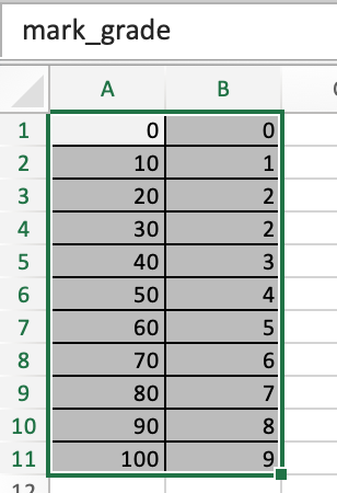
Note that the first column is sorted in ascending order. That's very important: the results become erratic and totally unreliable if you don't do that.
Now, to save a bit of hassle later, it's a good idea to name this table, so that you can refer it by name rather than cell references. Doing so is ridiculously easy: just select the table in the usual way, and then click in the name box, which usually shows a cell reference, and then type a name which describes the table, and press Enter. In this example, I've used the name mark_grade. Note the use of the underscore: spaces are not allowed.
Back to the main sheet. First off, name the cell ranges you will be using. To name the Mark column, click on the letter above it, and then in the name box type the name "Marks". That will name the whole column as "Marks".
Next, repeat this process for the Predicted Grade and Awarded Grade columns.
OK, we're now ready to roll.
In the first empty cell in the Predicted Grade column, enter this formula:
=VLOOKUP(marks,mark_grade,2)
What this means is:
Look at the value in the Marks column. Then look up this value in the first column of the table showing the marks and corresponding grades. Finally, read off the value shown in the second column of the table.
In practice this works well because the formula does not require an exact value. Thus, if the mark is 48, the formula will return a grade of D. But if the mark is anywhere between 50 and 59 (inclusive), it will return a grade C. In other words, it only changes grade when you reach the next cut-off point.
To copy the formula down, place the mouse pointer on the bottom right-hand corner of the cell and either double-click or drag it down.
The formula in the next column, ie Awarded Grade, is:
=predicted_grade
Where the student's actual performance in the mock exam be different to what was predicted, simply enter their actual grade, overriding the formula.
You can then set up Conditional Formatting to highlight the cells in the Actual Grade column that are different to those in the Predicted Grade column. (Bear in mind that if you are staring at a column of 200 grades the differences won't be immediately apparent, hence my suggestion of using Conditional Formatting.)
Interview the student concerned to ascertain the reason for the difference, and enter that in the Comments column.
So the completed spreadsheet will look something like this:

I can honestly say that this system saved me and my team hours and hours. Hope you enjoy using it.
Remember: if you can’t be bothered, or don’t have the time, to set this up yourself, then subscribe to my newsletter Digital Education The day after you subscribe you’ll receive a link to the newsletter’s supplement page, where you find a link to a file you can download and adapt for your own circumstances.